mcsm-benchs: Benchmarking methods for component retrieval

import numpy as np
from numpy import pi as pi
import scipy.signal as sg
import pandas as pd
from matplotlib import pyplot as plt
from mcsm_benchs.Benchmark import Benchmark
from mcsm_benchs.ResultsInterpreter import ResultsInterpreter
from mcsm_benchs.SignalBank import SignalBank
from utils import get_stft, invert_stft

Creating a dictionary of signals

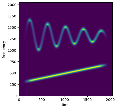
We can use the SignalBank class to generate a dictionary of signals to study. We are going to use a signal with two components: 1) a linear chirp, 2) a cosenoidal chirp. Below we can see how to generate the signal as well as its spectrogram.

We use the option return_signal=True, so that the signals generated by the SignalBank are objects of the Signal class, which behave like a regular numpy array, but include additional information of the generated signals, such as the instantaneous frequency of each signal component.

# Create a dictionary of signals:
N = 2048
sb = SignalBank(N=N, return_signal=True)

signal_1 = sb.signal_mc_damped_cos()

# Create a dictionary of signals for later.
signals = {'linear_chirp':signal_1,}

# Display the spectrograms of the signals.
stft1 = get_stft(signal_1)

fig, axs = plt.subplots(1,1, sharey=True)
axs.imshow(np.abs(stft1)**2, origin='lower')
axs.set_xlabel('time'); axs.set_ylabel('frequency')

Text(0, 0.5, 'frequency')

Creating a dictionary of methods

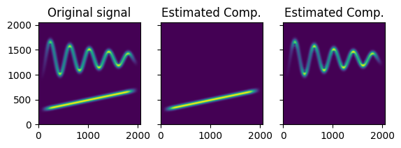
We define a simple method that tracks two ridges in the spectrogram as a chain of maxima for each column. After detecting a ridge, the method sets to \(0\) a number \(L\) of pixes above and below the ridge, allowing to search for another ridge using the residual STFT. This is known as a peeling scheme. Finding a particular value of \(L\) for a signal depends on the SNR of the component. \(2L\) is also the width of the strip of the STFT used to recover the individual components.

We will study the results for this only method but using different values of the parameter \(L\), and evaluate the reconstruction of each component.

The method should return a list of components, in any order. The benchmarking procedure takes care of matching the output of the method with the most similar component from the signal in order to compute the quality reconstruction factor (QRF) for each component.

def get_ridge(stft, L=100):
    """
    Get a ridge from the stft of a signal
    """
    spectrogram = np.abs(stft)**2
    stft2 = stft.copy()
    mask = np.zeros_like(spectrogram)
    ridge = np.zeros((spectrogram.shape[1]))
    for i in range(spectrogram.shape[1]):
        ridge[i] = np.argmax(spectrogram[:,i])
        stft2[int(np.max([0,ridge[i]-L])):int(np.min([ridge[i]+L,stft.shape[0]])),i] = 0 # Erase current ridge from spectrogram.
        mask[int(np.max([0,ridge[i]-L])):int(np.min([ridge[i]+L,stft.shape[0]])),i] = 1
    return ridge, stft2, mask

def method_1(signal, L=100):
    # 1. Compute STFT
    stft = get_stft(signal)
    # 2. Get two ridges from spectrogram
    resid_stft = stft
    components = []
    for i in range(2):
        ridge, resid_stft, mask = get_ridge(resid_stft, L=L)
        component = invert_stft(stft,mask=mask)
        components.append(component)
    return components # List of estimated components, even if its only one.

# Check results using one of the signals defined before.
components = method_1(signal_1, L=100) # Output of the method for L=100
fig, axs = plt.subplots(1,3, sharey=True)
axs[0].imshow(np.abs(get_stft(signal_1)), origin='lower')
axs[0].set_title('Original signal')
axs[1].imshow(np.abs(get_stft(components[0])), origin='lower')
axs[1].set_title('Estimated Comp.')
axs[2].imshow(np.abs(get_stft(components[1])), origin='lower')
axs[2].set_title('Estimated Comp.')

Text(0.5, 1.0, 'Estimated Comp.')

Finally, we create a dictionary of methods to compare (with only one method here), and a dictionary of parameters to use with each method.

methods = {'method_1':method_1,}
parameters = {'method_1':[
                        {'L':25},
                        {'L':50},
                        {'L':100},
                        ]
            }

Instantiating a benchmark object

We instantiate a benchmark object and run the tests.

benchmark = Benchmark(task='component_denoising',
                      methods=methods,
                      parameters=parameters,
                      signal_ids=signals,
                      SNRin=[0,10,20],
                      repetitions=5,
                      N = N,
                      verbosity=5)
benchmark.run()

Running benchmark...
- Signal linear_chirp
-- SNR: 0 dB
--- Method: method_1
---- Parameters Combination: 0
------ Inner loop. method_1: 0
------ Inner loop. method_1: 1
------ Inner loop. method_1: 2
------ Inner loop. method_1: 3
------ Inner loop. method_1: 4
Elapsed:1.598179817199707
---- Parameters Combination: 1
------ Inner loop. method_1: 0
------ Inner loop. method_1: 1
------ Inner loop. method_1: 2
------ Inner loop. method_1: 3
------ Inner loop. method_1: 4
Elapsed:1.5431218147277832
---- Parameters Combination: 2
------ Inner loop. method_1: 0
------ Inner loop. method_1: 1
------ Inner loop. method_1: 2
------ Inner loop. method_1: 3
------ Inner loop. method_1: 4
Elapsed:1.5588950157165526
-- SNR: 10 dB
--- Method: method_1
---- Parameters Combination: 0
------ Inner loop. method_1: 0
------ Inner loop. method_1: 1
------ Inner loop. method_1: 2
------ Inner loop. method_1: 3
------ Inner loop. method_1: 4
Elapsed:1.5767138004302979
---- Parameters Combination: 1
------ Inner loop. method_1: 0
------ Inner loop. method_1: 1
------ Inner loop. method_1: 2
------ Inner loop. method_1: 3
------ Inner loop. method_1: 4
Elapsed:1.5996645450592042
---- Parameters Combination: 2
------ Inner loop. method_1: 0
------ Inner loop. method_1: 1
------ Inner loop. method_1: 2
------ Inner loop. method_1: 3
------ Inner loop. method_1: 4
Elapsed:1.5932747364044189
-- SNR: 20 dB
--- Method: method_1
---- Parameters Combination: 0
------ Inner loop. method_1: 0
------ Inner loop. method_1: 1
------ Inner loop. method_1: 2
------ Inner loop. method_1: 3
------ Inner loop. method_1: 4
Elapsed:1.5435516834259033
---- Parameters Combination: 1
------ Inner loop. method_1: 0
------ Inner loop. method_1: 1
------ Inner loop. method_1: 2
------ Inner loop. method_1: 3
------ Inner loop. method_1: 4
Elapsed:1.5798948764801026
---- Parameters Combination: 2
------ Inner loop. method_1: 0
------ Inner loop. method_1: 1
------ Inner loop. method_1: 2
------ Inner loop. method_1: 3
------ Inner loop. method_1: 4
Elapsed:1.5917760848999023
The test has finished.

{'perf_metric': {'linear_chirp': {0: {'method_1': {"{'L': 25}": {'Comp.0': [np.float64(1.9345058847705467),
       np.float64(1.1282311561428875),
       np.float64(0.9410921708666034),
       np.float64(1.1546533420250624),
       np.float64(1.4987758767200394)],
      'Comp.1': [np.float64(5.175580885279313),
       np.float64(8.19876681693958),
       np.float64(5.286697485064469),
       np.float64(8.669357043621943),
       np.float64(7.650636930463604)]},
     "{'L': 50}": {'Comp.0': [np.float64(3.8208649938350403),
       np.float64(5.455134515150642),
       np.float64(3.607283581262556),
       np.float64(4.877066684972691),
       np.float64(4.666206191674506)],
      'Comp.1': [np.float64(4.319067525652214),
       np.float64(7.062947898884301),
       np.float64(4.230686571236454),
       np.float64(7.25084716698017),
       np.float64(6.686451720468276)]},
     "{'L': 100}": {'Comp.0': [np.float64(4.371009198299424),
       np.float64(6.050561048363743),
       np.float64(4.196274908796927),
       np.float64(5.666757338103646),
       np.float64(5.5084936329620735)],
      'Comp.1': [np.float64(3.2591057879819734),
       np.float64(5.345952599845003),
       np.float64(3.1022914571998377),
       np.float64(5.678273229334579),
       np.float64(5.222835953629762)]}}},
   10: {'method_1': {"{'L': 25}": {'Comp.0': [np.float64(3.1794853875344935),
       np.float64(2.4683056726803674),
       np.float64(2.282625013370526),
       np.float64(2.3343049140289445),
       np.float64(2.248433656167679)],
      'Comp.1': [np.float64(12.254898141264105),
       np.float64(14.77843208626979),
       np.float64(11.114214314875817),
       np.float64(14.938372153944979),
       np.float64(12.979656547432782)]},
     "{'L': 50}": {'Comp.0': [np.float64(9.041697553874679),
       np.float64(9.498485790327019),
       np.float64(8.185426251990938),
       np.float64(9.414451523075533),
       np.float64(8.903311988710318)],
      'Comp.1': [np.float64(15.100606969203373),
       np.float64(21.178905645081784),
       np.float64(12.579658650599498),
       np.float64(19.702890059788228),
       np.float64(15.907363628079459)]},
     "{'L': 100}": {'Comp.0': [np.float64(13.434171592022269),
       np.float64(15.220317449623126),
       np.float64(11.54238727037582),
       np.float64(15.254464616987079),
       np.float64(13.654549142188904)],
      'Comp.1': [np.float64(13.991942242839325),
       np.float64(17.74604283758289),
       np.float64(11.78177462908232),
       np.float64(17.230117982698566),
       np.float64(14.503241668406856)]}}},
   20: {'method_1': {"{'L': 25}": {'Comp.0': [np.float64(2.7916975519316036),
       np.float64(2.6709074018981456),
       np.float64(2.662176305585389),
       np.float64(2.5725156138052876),
       np.float64(2.542967232627133)],
      'Comp.1': [np.float64(14.87383862686157),
       np.float64(15.038587595103653),
       np.float64(14.904783776444251),
       np.float64(15.259010046466255),
       np.float64(15.074281252614457)]},
     "{'L': 50}": {'Comp.0': [np.float64(10.16005721906393),
       np.float64(10.017593755138872),
       np.float64(10.105618437252435),
       np.float64(10.013835257391541),
       np.float64(9.998069963273092)],
      'Comp.1': [np.float64(29.46580652383519),
       np.float64(30.68537702951093),
       np.float64(30.37218617952931),
       np.float64(30.902228088645174),
       np.float64(30.82719628692924)]},
     "{'L': 100}": {'Comp.0': [np.float64(18.88766168596554),
       np.float64(18.451550246682388),
       np.float64(18.70504935446653),
       np.float64(18.643398021731063),
       np.float64(18.526666568942503)],
      'Comp.1': [np.float64(27.156250258386887),
       np.float64(27.559718333920642),
       np.float64(27.21948425588033),
       np.float64(27.873369246766018),
       np.float64(27.636428429525353)]}}}}}}

Displaying results.

results = benchmark.results # Get dictionary with the results.
df = benchmark.dic2df(results) # Transform dictionary to DataFrame
df = df.reset_index()
df

	level_0	level_1	level_2	level_3	level_4	level_5	Comp.0	Comp.1
0	perf_metric	linear_chirp	0	method_1	{'L': 25}	0	1.934506	5.175581
1	perf_metric	linear_chirp	0	method_1	{'L': 25}	1	1.128231	8.198767
2	perf_metric	linear_chirp	0	method_1	{'L': 25}	2	0.941092	5.286697
3	perf_metric	linear_chirp	0	method_1	{'L': 25}	3	1.154653	8.669357
4	perf_metric	linear_chirp	0	method_1	{'L': 25}	4	1.498776	7.650637
5	perf_metric	linear_chirp	0	method_1	{'L': 50}	0	3.820865	4.319068
6	perf_metric	linear_chirp	0	method_1	{'L': 50}	1	5.455135	7.062948
7	perf_metric	linear_chirp	0	method_1	{'L': 50}	2	3.607284	4.230687
8	perf_metric	linear_chirp	0	method_1	{'L': 50}	3	4.877067	7.250847
9	perf_metric	linear_chirp	0	method_1	{'L': 50}	4	4.666206	6.686452
10	perf_metric	linear_chirp	0	method_1	{'L': 100}	0	4.371009	3.259106
11	perf_metric	linear_chirp	0	method_1	{'L': 100}	1	6.050561	5.345953
12	perf_metric	linear_chirp	0	method_1	{'L': 100}	2	4.196275	3.102291
13	perf_metric	linear_chirp	0	method_1	{'L': 100}	3	5.666757	5.678273
14	perf_metric	linear_chirp	0	method_1	{'L': 100}	4	5.508494	5.222836
15	perf_metric	linear_chirp	10	method_1	{'L': 25}	0	3.179485	12.254898
16	perf_metric	linear_chirp	10	method_1	{'L': 25}	1	2.468306	14.778432
17	perf_metric	linear_chirp	10	method_1	{'L': 25}	2	2.282625	11.114214
18	perf_metric	linear_chirp	10	method_1	{'L': 25}	3	2.334305	14.938372
19	perf_metric	linear_chirp	10	method_1	{'L': 25}	4	2.248434	12.979657
20	perf_metric	linear_chirp	10	method_1	{'L': 50}	0	9.041698	15.100607
21	perf_metric	linear_chirp	10	method_1	{'L': 50}	1	9.498486	21.178906
22	perf_metric	linear_chirp	10	method_1	{'L': 50}	2	8.185426	12.579659
23	perf_metric	linear_chirp	10	method_1	{'L': 50}	3	9.414452	19.702890
24	perf_metric	linear_chirp	10	method_1	{'L': 50}	4	8.903312	15.907364
25	perf_metric	linear_chirp	10	method_1	{'L': 100}	0	13.434172	13.991942
26	perf_metric	linear_chirp	10	method_1	{'L': 100}	1	15.220317	17.746043
27	perf_metric	linear_chirp	10	method_1	{'L': 100}	2	11.542387	11.781775
28	perf_metric	linear_chirp	10	method_1	{'L': 100}	3	15.254465	17.230118
29	perf_metric	linear_chirp	10	method_1	{'L': 100}	4	13.654549	14.503242
30	perf_metric	linear_chirp	20	method_1	{'L': 25}	0	2.791698	14.873839
31	perf_metric	linear_chirp	20	method_1	{'L': 25}	1	2.670907	15.038588
32	perf_metric	linear_chirp	20	method_1	{'L': 25}	2	2.662176	14.904784
33	perf_metric	linear_chirp	20	method_1	{'L': 25}	3	2.572516	15.259010
34	perf_metric	linear_chirp	20	method_1	{'L': 25}	4	2.542967	15.074281
35	perf_metric	linear_chirp	20	method_1	{'L': 50}	0	10.160057	29.465807
36	perf_metric	linear_chirp	20	method_1	{'L': 50}	1	10.017594	30.685377
37	perf_metric	linear_chirp	20	method_1	{'L': 50}	2	10.105618	30.372186
38	perf_metric	linear_chirp	20	method_1	{'L': 50}	3	10.013835	30.902228
39	perf_metric	linear_chirp	20	method_1	{'L': 50}	4	9.998070	30.827196
40	perf_metric	linear_chirp	20	method_1	{'L': 100}	0	18.887662	27.156250
41	perf_metric	linear_chirp	20	method_1	{'L': 100}	1	18.451550	27.559718
42	perf_metric	linear_chirp	20	method_1	{'L': 100}	2	18.705049	27.219484
43	perf_metric	linear_chirp	20	method_1	{'L': 100}	3	18.643398	27.873369
44	perf_metric	linear_chirp	20	method_1	{'L': 100}	4	18.526667	27.636428

Before displaying the results, we need to format the DataFrame in the correct way:

# For the first Component:
df = df.iloc[:,[3,4,1,5,2,6]]
col_names = list(df.columns)
col_names[0:6] = ['Method','Parameter', 'Signal_id','Repetition','SNR','QRF']
df.columns = col_names
df = df.pivot_table(index= ['Method','Parameter', 'Signal_id','Repetition'], columns='SNR', values='QRF')
df = df.reset_index()
df

SNR	Method	Parameter	Signal_id	Repetition	0	10	20
0	method_1	{'L': 100}	linear_chirp	0	4.371009	13.434172	18.887662
1	method_1	{'L': 100}	linear_chirp	1	6.050561	15.220317	18.451550
2	method_1	{'L': 100}	linear_chirp	2	4.196275	11.542387	18.705049
3	method_1	{'L': 100}	linear_chirp	3	5.666757	15.254465	18.643398
4	method_1	{'L': 100}	linear_chirp	4	5.508494	13.654549	18.526667
5	method_1	{'L': 25}	linear_chirp	0	1.934506	3.179485	2.791698
6	method_1	{'L': 25}	linear_chirp	1	1.128231	2.468306	2.670907
7	method_1	{'L': 25}	linear_chirp	2	0.941092	2.282625	2.662176
8	method_1	{'L': 25}	linear_chirp	3	1.154653	2.334305	2.572516
9	method_1	{'L': 25}	linear_chirp	4	1.498776	2.248434	2.542967
10	method_1	{'L': 50}	linear_chirp	0	3.820865	9.041698	10.160057
11	method_1	{'L': 50}	linear_chirp	1	5.455135	9.498486	10.017594
12	method_1	{'L': 50}	linear_chirp	2	3.607284	8.185426	10.105618
13	method_1	{'L': 50}	linear_chirp	3	4.877067	9.414452	10.013835
14	method_1	{'L': 50}	linear_chirp	4	4.666206	8.903312	9.998070

Finally, we can use the functionality from the ResultsInterpreter class to display the result on interactive plots (using plotly).

# Summary interactive plots with Plotly and a report.
from plotly.offline import  iplot
import plotly.io as pio
pio.renderers.default = "plotly_mimetype+notebook"
interpreter = ResultsInterpreter(benchmark)
figs = interpreter.get_summary_plotlys(df, bars=True,)
for fig in figs:
    iplot(fig)

results = benchmark.results # Get dictionary with the results.
df = benchmark.dic2df(results) # Transform dictionary to DataFrame
df = df.reset_index()

# For the second component:
df = df.iloc[:,[3,4,1,5,2,7]]
col_names = list(df.columns)
col_names[0:6] = ['Method','Parameter', 'Signal_id','Repetition','SNR','QRF']
df.columns = col_names
df = df.pivot_table(index= ['Method','Parameter', 'Signal_id','Repetition'], columns='SNR', values='QRF')
df = df.reset_index()
df

SNR	Method	Parameter	Signal_id	Repetition	0	10	20
0	method_1	{'L': 100}	linear_chirp	0	3.259106	13.991942	27.156250
1	method_1	{'L': 100}	linear_chirp	1	5.345953	17.746043	27.559718
2	method_1	{'L': 100}	linear_chirp	2	3.102291	11.781775	27.219484
3	method_1	{'L': 100}	linear_chirp	3	5.678273	17.230118	27.873369
4	method_1	{'L': 100}	linear_chirp	4	5.222836	14.503242	27.636428
5	method_1	{'L': 25}	linear_chirp	0	5.175581	12.254898	14.873839
6	method_1	{'L': 25}	linear_chirp	1	8.198767	14.778432	15.038588
7	method_1	{'L': 25}	linear_chirp	2	5.286697	11.114214	14.904784
8	method_1	{'L': 25}	linear_chirp	3	8.669357	14.938372	15.259010
9	method_1	{'L': 25}	linear_chirp	4	7.650637	12.979657	15.074281
10	method_1	{'L': 50}	linear_chirp	0	4.319068	15.100607	29.465807
11	method_1	{'L': 50}	linear_chirp	1	7.062948	21.178906	30.685377
12	method_1	{'L': 50}	linear_chirp	2	4.230687	12.579659	30.372186
13	method_1	{'L': 50}	linear_chirp	3	7.250847	19.702890	30.902228
14	method_1	{'L': 50}	linear_chirp	4	6.686452	15.907364	30.827196

# Summary interactive plots with Plotly and a report.
from plotly.offline import  iplot
import plotly.io as pio
pio.renderers.default = "plotly_mimetype+notebook"
interpreter = ResultsInterpreter(benchmark)
figs = interpreter.get_summary_plotlys(df, bars=True,)
for fig in figs:
    iplot(fig)