mcsm-benchs: Querying Signal class attributes for more versatile benchmarks

The SignalBank class encapsulates the signal generation code and yields a dictionary with a number of signals. In order to access those signals, the keys of this dictionary are called signal_id. The constructor simply takes the number N of samples of the desired signals.

Within the Benchmark class, the signals obtained from the SignalBank class are given as objects of another custom class called Signal. This class behaves like a regular numpy array, but it also comprises a series of attributes of the signal that some methods might need. Moreover, benchmarks can be built to estimate these quantities as well.

Let’s see some examples.

import numpy as np
import scipy.signal as sg
from numpy import pi as pi
from matplotlib import pyplot as plt
from mcsm_benchs.SignalBank import SignalBank
from mcsm_benchs.Benchmark import Benchmark
from mcsm_benchs.ResultsInterpreter import ResultsInterpreter
from utils import get_stft

# plt.rcParams['image.cmap'] = 'binary'

# Set the length of the signals to generate
N = 1024

# The second parameter makes it return objects of the Signal class
signal_bank = SignalBank(N=N, return_signal=True)
signal_dic = signal_bank.generate_signal_dict()

# Select three signals as examples:
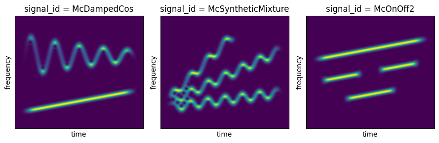
signal_ids = ['McDampedCos','McSyntheticMixture', 'McOnOff2']

# Plot the spectrograms of some signals:
fig, ax = plt.subplots(1, 3, layout='tight', figsize=(9,3))

for i,signal_id in enumerate(signal_ids):
    signal = signal_dic[signal_id]
    S = np.abs(get_stft(signal))**2
    idx = np.unravel_index(i, ax.shape)
    ax[idx].imshow(S, origin = 'lower',aspect='auto')
    ax[idx].set_title('signal_id = '+ signal_id)
    ax[idx].set_xticks([],[])
    ax[idx].set_xlabel('time')
    ax[idx].set_yticks([])
    ax[idx].set_ylabel('frequency')

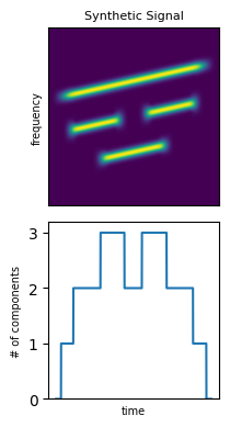
We can now query a Signal instance to obtain:

• Total number of components

• Number of components at each time instant

• Instantaneous frequency of each component

• Each individual component

signal_1 = signal_dic[signal_ids[2]]
print('Total number of components: {}'.format(signal_1.total_comps))

fig, axs = plt.subplots(2, 1, layout='tight', figsize=(2.2,4))
S = np.abs(get_stft(signal_1))
axs[0].imshow(S, origin = 'lower',aspect='auto')
# axs[0].set_title('signal_id = '+ signal_ids[2])
axs[0].set_title('Synthetic Signal', fontsize=8)
axs[0].set_xticks([],[])
# axs[0].set_xlabel('time')
axs[0].set_yticks([])
axs[0].set_ylabel('frequency',fontsize=7)

# Plot the instantaneous frequencies on top
# for instafreq in signal_1.instf:
#     axs[0].plot(instafreq*2*N,'--')

axs[1].plot(signal_1.ncomps)
axs[1].set_xlabel('time', fontsize=7)
axs[1].set_ylabel('# of components',fontsize=7)
axs[1].set_ylim([0,3.2])
axs[1].set_yticks([0,1,2,3])
axs[1].set_xticks([],[])


# fig.savefig('signals_ncomps.pdf',dpi=900, transparent=False,bbox_inches='tight')

Total number of components: 4

[]

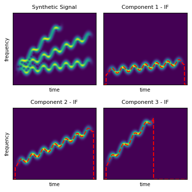
We can also get the separated components of a signal

signal_2 = signal_dic[signal_ids[1]]
print(type(signal_2))
print('Total number of components: {}'.format(signal_2.total_comps))

# Plot the spectrograms of some signals:
fig, ax = plt.subplots(2, 2, sharex=True,sharey=True, layout='tight', figsize=(4,4))
idx = np.unravel_index(0, ax.shape)
S = np.abs(get_stft(signal_2))
ax[idx].imshow(S, origin = 'lower',aspect='auto')
ax[idx].set_title('Synthetic Signal',fontsize=8)
ax[idx].set_xticks([],[])
ax[idx].set_xlabel('time', fontsize=7)
ax[idx].set_yticks([])
ax[idx].set_ylabel('frequency', fontsize=7)


for i in range(1,signal_2.total_comps+1):
    component = signal_2.comps[i-1]
    S = np.abs(get_stft(component))
    idx = np.unravel_index(i, ax.shape)
    ax[idx].imshow(S, origin = 'lower',aspect='auto')
    ax[idx].set_title('Component {} - IF'.format(i),fontsize=8)
    ax[idx].set_xticks([],[])
    ax[idx].set_xlabel('time', fontsize=7)
    ax[idx].set_yticks([])
    if np.mod(i,2)==0:
        ax[idx].set_ylabel('frequency', fontsize=7)
    ax[idx].plot(signal_2.instf[i-1]*2*N,'r--')

# fig.savefig('signals_ifs.pdf',dpi=900, transparent=False,bbox_inches='tight')

<class 'mcsm_benchs.SignalBank.Signal'>
Total number of components: 3

Benchmarking a component counting method

methods = {'fun1': lambda x,*args,**kwargs: 4,
            'fun2': lambda x,*args,**kwargs: x.total_comps,
            }

perf_fun = {'Error': lambda x, x_hat, *args, **kwargs: x.total_comps-x_hat,}


benchmark = Benchmark(task = 'misc',
                        methods = methods,
                        N = 256,
                        SNRin = [10,20],
                        repetitions = 3,
                        obj_fun=perf_fun,
                        signal_ids=['LinearChirp', 'CosChirp',],
                        verbosity=0,
                        parallelize=False,
                        )

benchmark.run() # Run the test. my_results is a dictionary with the results for each of the variables of the simulation.
benchmark.save_to_file('saved_benchmark') # Save the benchmark to a file.

Running benchmark...

100%|██████████| 2/2 [00:00<00:00, 1592.37it/s]
100%|██████████| 2/2 [00:00<00:00, 1758.25it/s]

True

benchmark = Benchmark.load_benchmark('saved_benchmark')
results_df = benchmark.get_results_as_df() # This formats the results on a DataFrame
results_df

	Method	Parameter	Signal_id	Repetition	10	20
6	fun1	((), {})	CosChirp	0	-3	-3
7	fun1	((), {})	CosChirp	1	-3	-3
8	fun1	((), {})	CosChirp	2	-3	-3
0	fun1	((), {})	LinearChirp	0	-3	-3
1	fun1	((), {})	LinearChirp	1	-3	-3
2	fun1	((), {})	LinearChirp	2	-3	-3
9	fun2	((), {})	CosChirp	0	0	0
10	fun2	((), {})	CosChirp	1	0	0
11	fun2	((), {})	CosChirp	2	0	0
3	fun2	((), {})	LinearChirp	0	0	0
4	fun2	((), {})	LinearChirp	1	0	0
5	fun2	((), {})	LinearChirp	2	0	0